[Python] Law of Large Numbers: Dice Roll

So Einstein was wrong when he said, “God does not play dice.” Consideration of black holes suggests, not only that God does play dice, but that he sometimes confuses us by throwing them where they can’t be seen.

Stephen Hawking

Photo by Aliko Sunawang from Pexels

I would recommend reading this post about the Law of Large Numbers before continuing with this one:

I want to run a quick and easy experiment which is in line with the Law of Large Numbers. That is to roll a dice for several times and see whether the average converges to the true value. One would expect that with more trials, the average of all dice rolls should converge to the true value, which is 3.5. Let’s see if that is actually the case.

Here is how it goes: A dice will be rolled several times, and the cumulative average is going to be calculated for every toss.

# Econowmics.com

#Importing the modules that I want
#This modules helps me produce random numbers
import random
#I will use this module to plot the graphs I want
import matplotlib.pyplot as plt 
#I need the numpy module because I was lazy to write a function to calculate the cumulative sum :D
import numpy as np

#Setting the seed
random.seed(1991)

#Defining a function for rolling the dice
def Roll(n):
    """This function simulates rolling a dice for n-times"""
    
    #Empty vector to store the result of dice roll
    result = []
    
    for i in range(1,n+1):
        result.append(random.choice([1, 2, 3, 4, 5, 6]))
    return result


#Now, lets roll the dice for a certain amount of times
result = Roll(1000000)

#Now, I want to plot how the average of dice rolls converge to the expected value (3.5)
#Empty list to store the values of averages
averages = []

_cumsum = np.cumsum(result)
for index in range(len(_cumsum)):
    averages.append(_cumsum[index]/(index+1))

#Plotting the averages
plt.plot(averages)

#Adding information to the graph
plt.xlabel('Trials') #naming the x-axis
plt.ylabel('Average of all outcomes') #naming the y-axis 
plt.title('Average value of Dice rolled ') #Graph title

This code is very simple. First, I have created a function which simulates rolling a dice: The function randomly chooses a number from all possible outcomes of a coin toss: [1, 2, 3, 4, 5, 6]). The function will then add the results to a pre-defined vector, which I will later use to calculate the averages from. Then the cumulative sum of the results is calculated with Numpy’s cumsum function, so that the averages can be calculated. A graph shows the final results.

#10 Trials

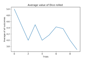
After just 10 trials, the average is already converging very quickly, standing at 3.8. First dice roll was a 5.

#100 Trials

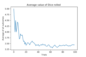
With 100 rolls, the average is already very close to true value.

#1000 Trials

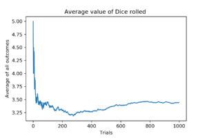
After 100 trials the average falls to about 3.25 and then again converges to 3.5.

#1000000 Trials

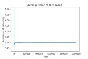
With one million dice rolls, the average is very very close to the true value, being 3.4998015132783884